
Ritika Chopra
Gagan Deep Sharma
Gagan Deep Sharma
University School of Management Studies, Guru Gobind Singh Indraprastha University, Dwarka Sector 16-C, New Delhi 110078, India
Author to whom correspondence should be addressed. J. Risk Financial Manag. 2021, 14(11), 526; https://doi.org/10.3390/jrfm14110526Submission received: 13 September 2021 / Revised: 16 October 2021 / Accepted: 18 October 2021 / Published: 4 November 2021
(This article belongs to the Special Issue Technical Analysis of Financial Markets)The stock market is characterized by extreme fluctuations, non-linearity, and shifts in internal and external environmental variables. Artificial intelligence (AI) techniques can detect such non-linearity, resulting in much-improved forecast results. This paper reviews 148 studies utilizing neural and hybrid-neuro techniques to predict stock markets, categorized based on 43 auto-coded themes obtained using NVivo 12 software. We group the surveyed articles based on two major categories, namely, study characteristics and model characteristics, where ‘study characteristics’ are further categorized as the stock market covered, input data, and nature of the study; and ‘model characteristics’ are classified as data pre-processing, artificial intelligence technique, training algorithm, and performance measure. Our findings highlight that AI techniques can be used successfully to study and analyze stock market activity. We conclude by establishing a research agenda for potential financial market analysts, artificial intelligence, and soft computing scholarship.
Stock prediction focuses on estimating the future price movement in a stock, which is generally perceived as a challenging task due to the non-stationarity and volatility of the stock data. Dynamic stock market price variation and its chaotic behavior have increased the price prediction problem where the extreme non-linear, dynamic, complicated domain knowledge inherent in the stock market has hiked the difficulty level for investors in making prompt investment decisions (Esfahanipour and Aghamiri 2010; Knill et al. 2012).
There are two traditional theories to take into account when estimating the stock price, namely, efficient market hypotheses (EMH) and random walk (RW) theory. EMH states that a stock price absorbs all known market knowledge at any time. Since market participants optimally use all known information, price fluctuations are unpredictable, as new information happens randomly (Fama 1970). Whereas according to the random walk theory, stock prices conduct a ‘random walk’, which means that all future prices do not follow any trends or patterns, and are a spontaneous deviation from previous prices, and an investor cannot possibly forecast the market (Cheng and Deets 1971; Van Horne and Parker 1967). Another model that challenges EMH is Paul Samuelson’s martingale model (Samuelson 1973), according to which, given all available information, current prices are the best predictors of an event’s outcome. The only significant predictor of the ultimate outcome, in particular, should be the most recent observed value (Richard and Vecer 2021).
The validity of the EMH and RW theory have been controversial. Therefore, with the emergence of computational and smart finance, and behavioral finance, economists have tried to establish another theory referred to as the inefficient market hypothesis (IMH), which states that financial markets are not always considered efficient markets. Market inefficiencies exist due to market psychology, transaction costs, information asymmetries, and human emotions (Asadi et al. 2012). The majority of studies have used AI techniques to support those arguments, and the fact that certain players can consistently outperform the market demonstrates that the EMH might not be entirely accurate in practice (Asadi et al. 2012). As a viable alternative to the EMH, the fractal market hypothesis (FMH) has also been established (Dar et al. 2017) by Peters (1994). According to the FMH, markets are stabilized by matching the demand and supply of investors’ investment horizons, whereas the EMH supposes that markets are in equilibrium (Dar et al. 2017; Karp and Van Vuuren 2019).
FMH examines the market’s daily randomness and the turbulence experienced during crashes and crises, and provides a compelling explanation for investor behavior over the course of a market cycle, including booms and busts (Moradi et al. 2021). Interestingly, it also considers the non-linear relationships in time series problems, hence making it a suitable theory for stock prediction and other time series (Aslam et al. 2021; Kakinaka and Umeno 2021; Naeem et al. 2021; Tilfani et al. 2020), or financial market related problems (Anderson and Noss 2013; Kumar et al. 2017; Singh et al. 2013). Nowadays, the value and benefits of forecasting in decision- and policy-making are unquestionably recognized across multiple dimensions. Naturally, the techniques that encounter the least amount of forecasting errors will survive and function properly (Moradi et al. 2021). Henceforth, many individuals, including academics, investment professionals, and average investors or traders, are actively searching for this superior system that will deliver high returns.
Stock price prediction based on time series of relevant variables and behavioral patterns (Khan et al. 2020a) helps determine prediction efficiency (Zahedi and Rounaghi 2015). Accurate modelling requires considering external phenomena that include recession or expansion periods and high- or low-volatility periods driven by cyclical and other short-term fluctuations in aggregate demand (Atsalakis and Valavanis 2009b). One of the essential requirements for anyone related to economic environments is to correctly predict market price changes and make correct decisions based on those predictions. Stock-market predictions have been a prevalent research topic for many years. The financial benefit may be considered the most critical problem of stock-market prediction. When a system can reliably select winners and losers in the competitive market environment, it will generate more income for the system owner.
This problem calls for developing intelligent systems for fetching real-time pricing information, which can enhance the profit-maximization for investors (Esfahanipour and Aghamiri 2010). Several intelligent systems or AI techniques have been developed in recent years for decision support, modelling expertise, and complicated automation tasks, including artificial networks, genetic algorithms, support vector machines, machine learning, probabilistic belief networks, and fuzzy logic (Chen et al. 2005; Sharma et al. 2020). Among all these techniques, artificial neural networks (ANNs) are widely popular across the fields mainly due to their ability to analyze complex non-linear relationships between input and output variables directly by learning the training data (Baba and Suto 2000). The characteristic of ANNs in providing models for a large class of real systems has attracted the attention of researchers seeking to apply ANNs to various decision support systems. Nevertheless, despite growing concerns for ANNs utilization, only limited success has been achieved so far mainly due to the random behavior and complexity of the stock market (Baba and Suto 2000).
Several studies have examined stock price forecasting using artificial intelligence. For e.g., Atsalakis and Valavanis (2009b) reviewed around 100 studies focusing on neural and neuro-fuzzy techniques applied to forecast stock markets; Bahrammirzaee (2010) conducted a comparative research review of three popular artificial intelligence techniques, i.e., expert systems, artificial neural networks, and hybrid intelligent systems, applied in finance; Gandhmal and Kumar (2019) systematically analyzed and reviewed stock market prediction techniques; Strader et al. (2020) also systematically reviewed relevant publications from the past twenty years, and classified them based on similar methods and contexts; and Obthong et al. (2020) surveyed machine learning algorithms and techniques for stock price prediction. While these contributions illuminated broad aspects of stock predictability problems using AI, only a few papers focused on how stock forecasting using AI analysis has appeared and evolved in recent decades (Fouroudi et al. 2020).
Our study is beneficial to stock traders, brokers, corporations, investors, and the government, as well as financial institutions, depositories, and banks. Successful AI-based models can assist stock traders, brokers, and investors in achieving massive gains that previously appeared impossible. When financial markets become more predictable, more investors will invest with confidence, allowing businesses to raise additional funds (via stock markets) to repay debt, launch new goods, and expand operations. As a result, consumer and corporate confidence will increase, which will benefit the broader economy (Müller 2019). Depositories will also see an increase in business as a result of the enlarged investor base. Increased investment in financial markets results in increased tax collections, which benefits the government (Neuhierl and Weber 2017). Increased money flow from investors or traders will also help financial institutions such as banks, mutual fund organizations, insurance businesses, and investment corporations (Neuhierl and Weber 2017; Škrinjarić and Orloví 2020). Additionally, just 0.128 percent of the world’s population trades or invests in the stock market—the remainder either lack access to the internet, or lack understanding of financial trading (Asktraders 2020). The majority of active traders and investors are afraid of trading and investing in financial markets because they lack the ability to appropriately forecast stock values due to market volatility (Smales 2017). As a result, they need to adopt an excellent forecasting model to instil investor trust and make massive profits (Hao and Gao 2020). We claim, in this review, that successful technology, supported by new AI-based models, can assist stock traders, brokers, and investors in attaining a competitive edge, which previously seemed unattainable.
Our study contributes by providing a coherent presentation and classification of artificial intelligence methods applied to various financial markets, which can be used for further analysis and comparison, as well as comparative studies. Moreover, our study also provides detailed future avenues on ‘feature selection algorithms’, ‘prediction range’ (long-term, short-term, and very short-term (minute-wise/hour-wise)), ‘stock markets covered’, ‘data pre-processing techniques’, ‘prediction forms’ (one-step-ahead and multiple-steps-ahead), and ‘performance measures’.
Additionally, the literature on the usage of artificial intelligence and soft computing techniques for stock market prediction is yet to develop an accurate predictive model (Zhou et al. 2019). One, the selection of input data is not rigorous in the majority of the studies leading to flawed model simulations and series estimations (Bildirici and Ersin 2009; Dhenuvakonda et al. 2020; Zhang et al. 2021). Two, the extant literature is, at best, partially successful in optimizing the parameter selections and model architectures (Tealab 2018). Three, the pre-processing of input data has not been carried out with precision in the extant literature so far (Atsalakis and Valavanis 2009b). To consolidate the extant literature and direct it towards developing a robust AI-based stock prediction model, we carry out this systematic literature review of papers listed on the Web of Science (WoS) and Scopus databases.
We begin by presenting an organizing framework classifying the extant literature into two major categories: study characteristics and model characteristics, where ‘study characteristics’ is further classified into the stock market covered, input data, and nature of the study; and ‘model parameter’ is grouped as data pre-processing, artificial intelligence technique, training algorithm, and performance measure (Figure 1). Our organizing framework is paralleled with a cohesive presentation of AI techniques employed on stock market predictions that can be used as a reference for future analysis and evaluation.
The rest of the paper is structured in the following manner. The second section represents the methodology of the paper outlining the keywords searched, acceptance criteria applied, and categorization framework. The third section outlays the trends and general description of the existing literature. The fourth section provides the results of this paper, as well as the thematic discussion that discusses the categories and subcategories. The fifth section and sixth section portray the gaps in the extant literature and the future research agenda, respectively. The last section concludes the paper.
The study’s methodology is influenced by Bansal et al. (2019) and Tranfield et al. (2003), and involves a rigorous review protocol enabling a high level of transparency and replicability. The search was conducted in May 2021 on the WoS and Scopus database(s) after identifying keywords (search terms) related to the artificial intelligence techniques in the title. The keywords used are ‘neur*’, ‘artificial*’, ‘AI’, ‘machine learning’, ‘deep learning’, ‘fuzzy’, ‘soft computing’, ‘forecast*’, ‘predict*’, ‘estimate*’, ‘stock market’, ‘stock return’, ‘stock price’, ‘share return’, ‘share market’, ‘share price’, ‘index return’, ‘index price’, along with the required Boolean operators (‘AND’, ‘OR’, ‘NOT’, ‘NEAR’, ‘W/n’, etc.). Both the WoS and Scopus databases are referred to the search for relevant articles due to their multidisciplinary nature, and easier access to literature belonging to economics, finance, management, psychology, technology, etc., enabling them to attain the most significant and latest studies. Moreover, both the databases have good coverage, which goes back to 1990, compared to other databases (Jain et al. 2019). We set the limit for the search to articles published between 1989 and 2021 (Rosado-Serrano et al. 2018). The papers are only extracted and evaluated if they are indexed by WoS and Scopus (for high credibility), written in English (for correct interpretation), and matched to the query as specified, whereas the remainder of the papers are declined.
This query yielded us 283 papers (152 from WoS; 131 from Scopus) initially, which were filtered for duplicates, leaving us with 202 records. These records were screened twice, leading to the elimination of 24 articles in the first screening process based on titles and abstracts only, as they belonged to different research areas, such as neural sciences, psychology, etc. Further, in the second screening process, 30 more articles were rejected (as they were not related to neural, hybrid-neuro, and stock market prediction), this time by thoroughly analyzing the full text of 178 papers, as they did not focus on applying artificial intelligence technique to forecast stock markets. This task left us with 148 articles in total, as presented in the PRISMA diagram (Moher et al. 2009) in Figure 2.
After shortlisting 148 papers, we divided the entire literature into major and minor categories, only based on 43 auto-coded themes (as given in Table 1) generated with the help of NVivo 12 software. For example, themes such as ‘daily’, ‘index’, ‘market’, ‘price’, ‘returns’, ‘stock’, ‘stock market’, ‘stock price’, ‘time’, and ‘time series’ are categorized as ‘stock market covered’; whereas ‘data’, ‘financial’, ‘information’, ‘input’, ‘parameters’, ‘value’, and ‘variables’ are categorized as ‘input data’; and ‘algorithm’ is categorized as ‘training algorithm’, etc.
The above auto-coded themes are categorized into study characteristics and model characteristics. Study characteristics are further categorized as the stock market covered, input data, and nature of the study. Model characteristics are classified as data pre-processing, artificial intelligence technique, training algorithm, and performance measure. Study characteristics give a glimpse of the stock markets covered, the type of input variables used, and whether or not the author has undertaken a comparative analysis of different AI techniques. Model characteristics detail the forecasting methodology used in the extant literature, including data pre-processing, artificial intelligence techniques employed, training algorithm applied, and performance measures (statistical or non-statistical) used to compare the performance of different models.
Additionally, we also downloaded the text and CSV files (full record and cited references) of 148 papers from both the databases, which included bibliographic data such as title, publication year, source journal, keywords, abstract, authors, authors’ addresses, subject categories, and references (van Nunen et al. 2018). We utilised this text file to employ scientometric or bibliometric analysis using the famous bibliometrix R-tool package (Aria and Cuccurullo 2017). Bibliometric techniques focused on portraying the publication history, the characteristics, and the scientific output advancement within a specific research area (Fouroudi et al. 2020). In our study, we have fetched data related to most contributing countries (Table 2), most relevant authors (Table 3), publications (Table 4), and journals (Table 5) using the bibliometrics R-tool, which is explained in the following sections.
Figure 3 summarizes the year-by-year publications and citations of papers relevant to the study’s subject. The research in applying AI techniques in stock market forecasting has significantly increased after 2008, representing a clear increasing trend in the related topic. This could be due to the global economic crisis of 2008 (Caporale et al. 2021), which made stock markets highly volatile, hence, attracting the widespread interest of research scholars and academicians in the discussed topic. The highest citation record is seen in the year 2020, with a 1377 citation record count.
Table 2 presents the top ten most contributing or productive countries, along with their international collaboration and citation analysis in the area of stock market prediction using AI. The documents retrieved were written by authors from 27 different countries. China was the most prolific publisher, followed by India, the USA, and Japan. Nonetheless, China (total citations = 1173) is unquestionably the leader in terms of total citations, as well as productivity (number of published articles = 42 (28.37 percent)). Five countries (i.e., Japan, Iran, Korea, Brazil, Australia in Table 2) hosted authors who published in the stock prediction using AI area (ergo, isolated countries in a collaboration aspect). In comparison, the remainder had at least one study that was published in multiple countries, where China (7) has the largest multi-country publications. The reason for this can be attributed to the growing emphasis on research and development, as well as increasing funding opportunities, in the country (Jia et al. 2021).

| Country | Articles | SCP | MCP | Citations |
|---|---|---|---|---|
| China | 42 | 35 | 7 | 1173 |
| India | 16 | 14 | 2 | 307 |
| USA | 16 | 12 | 4 | 714 |
| Japan | 9 | 9 | 0 | 126 |
| Turkey | 7 | 6 | 1 | 571 |
| Greece | 6 | 3 | 3 | 516 |
| Iran | 6 | 6 | 0 | 351 |
| Korea | 5 | 5 | 0 | 425 |
| Brazil | 4 | 4 | 0 | 182 |
| Australia | 3 | 3 | 0 | 17 |
Table 3 provides a list of the ten most prolific writers who contributed at least one publication between 1989 and 2021, sorted by cumulative citations earned. The research impact is determined with the help of three author level metrics, namely: h-index; g-index; and m-index. H-index is computed by totaling the publication count for which an author has been cited by other authors at least that same number of times (Hirsch 2005). G-index calculates the distribution of citations received by an author’s publications, depicting the performance of researchers’ top articles (Mazurek 2017). M-index is the median number of citations computed as h/n, where n is the number of years since the first published paper of the author, and is also called the m-quotient (Bornmann et al. 2008). ‘Atsalakis, G. S,’ sits on the top of the list with the highest publication count, the number of citations (473), h-index (4), g-index (4), and m-index (0.308).
| Rank | Author | h_index | g_index | m_index | Total Citations | No. of Publications | Publication Year Start |
|---|---|---|---|---|---|---|---|
| 1 | Atsalakis, G. S. | 4 | 4 | 0.308 | 473 | 4 | 2009 |
| 2 | Valavanis, K. P. | 3 | 3 | 0.231 | 443 | 3 | 2009 |
| 3 | Kim, K. J. | 2 | 2 | 0.091 | 361 | 2 | 2000 |
| 4 | Han, I. | 1 | 1 | 0.045 | 325 | 1 | 2000 |
| 5 | Hadavandi, E. | 3 | 3 | 0.25 | 303 | 3 | 2010 |
| 6 | Baykan, O. K. | 1 | 1 | 0.091 | 219 | 1 | 2011 |
| 7 | Boyacioglu, M. A. | 1 | 1 | 0.091 | 219 | 1 | 2011 |
| 8 | Kara, Y. | 1 | 1 | 0.091 | 219 | 1 | 2011 |
| 9 | Daim, T. U. | 1 | 1 | 0.091 | 212 | 1 | 2011 |
| 10 | Guresen, E. | 1 | 1 | 0.091 | 212 | 1 | 2011 |
Table 4 depicts the top ten cited publications arranged according to the total citations received. Kim and Han (2000) lead in citation count (325 citations), representing high relevance to the content of this document, i.e., various genetic algorithms approaches featuring discretization in artificial neural networks for stock price index prediction, whereas Atsalakis and Valavanis (2009b), who present a survey of soft computing methods used for stock market forecasting, have received the highest number of total citations per year.
| Rank | Publication | Total Citations (TC) | TC per Year |
|---|---|---|---|
| 1 | (Kim and Han 2000) | 325 | 14.7727 |
| 2 | (Atsalakis and Valavanis 2009b) | 295 | 22.6923 |
| 3 | (Kara et al. 2011) | 219 | 19.9091 |
| 4 | (Guresen et al. 2011) | 212 | 19.2727 |
| 5 | (Chen et al. 2003) | 204 | 10.7368 |
| 6 | (Enke and Thawornwong 2005) | 187 | 11 |
| 7 | (Yudong and Wu 2009) | 186 | 14.3077 |
| 8 | (Hadavandi et al. 2010) | 176 | 14.6667 |
| 9 | (Ticknor 2013) | 173 | 19.2222 |
| 10 | (Hsieh et al. 2011) | 173 | 15.7273 |
Table 5 shows the top 20 impactful journals publishing in the area of stock market prediction using AI over the last three decades, along with their h, g, and m index. ‘Expert Systems with Applications’ is the top journal in the list, with the highest number of publications (23), highest h-index (20), g-index (23), m-index (0.909), and citation count (2414), even though its publication start year is 2000. This is indicative of the growing interest of researchers in the field of AI applicability in different areas post-2000 (Johari 2020), and the significance of ‘Expert Systems with Applications’ in the creation and sharing of knowledge in this field.
| Rank | Source | h_index | g_index | m_index | Total Citations | No. of Publications | Publication Year Start |
|---|---|---|---|---|---|---|---|
| 1 | Expert Systems with Applications | 20 | 23 | 0.909 | 2414 | 23 | 2000 |
| 2 | Applied Soft Computing | 8 | 10 | 0.727 | 472 | 10 | 2011 |
| 3 | Computers & Operations Research | 2 | 2 | 0.105 | 280 | 2 | 2003 |
| 4 | Knowledge-Based Systems | 2 | 2 | 0.167 | 252 | 2 | 2010 |
| 5 | Neurocomputing | 4 | 4 | 0.154 | 140 | 4 | 1996 |
| 6 | International Journal of Forecasting | 2 | 2 | 0.083 | 122 | 2 | 1998 |
| 7 | Journal of Business Research | 1 | 1 | 0.056 | 79 | 1 | 2004 |
| 8 | Neural Computing & Applications | 4 | 8 | 0.041 | 64 | 8 | 1996 |
| 9 | Journal of Retailing | 1 | 1 | 0.038 | 61 | 1 | 1996 |
| 10 | Plos One | 2 | 4 | 0.286 | 53 | 4 | 2015 |
This section comprehends the extant literature concerning the stock markets covered, the type of input variables used, and the usage of comparative analysis.
The extant literature explores different world indices and stock markets to extract the input data directly or indirectly, to train and test their model (Atsalakis and Valavanis 2009b), and subsequently, predict the future prices. Some studies focus on predicting the stock indices at particular points in time, to offer conclusions regarding the related risks, thereby raising questions on the reliability of market robustness for highly successful investments. Such cases can significantly contribute towards vital information about accurate forecasting of models, stock markets, and stock returns (Atsalakis 2014).
This category is designed according to the world continents coded as sub-categories (Europe, Asia, Oceania, America, and Africa) (as given in Table A1). The surveyed stock indices from developed markets include Standard and Poor’s 500 (S & P 500), the Dow Jones Industrial Average (DJIA), New York Stock Exchange (NYSE), and National Association of Securities Dealers Automated Quotations (NASDAQ) from: the USA (Chenoweth and Obradović 1996; Donaldson and Kamstra 1999); the Tokyo Stock Exchange Index (TOPIX) and NIKKEI in Japan (Bekiros 2007; Dai et al. 2012); the Financial Times Stock Exchange 100 Share (FTSE) in London (Kanas 2001; Kanas and Yannopoulos 2001; Vella and Ng 2014); the main German Stock Exchange index, DAX (Hafezi et al. 2015; Rast 1999; Siekmann et al. 2001; Vella and Ng 2014); the Toronto stock exchange (TSX) indices in Canada (Olson and Mossman 2003); the Australian stock exchange index (ASX) in Australia (Pan et al. 2005; Vanstone et al. 2005); and the New Zealand stock index (NZX-50) in New Zealand (Fong et al. 2005). Among all the developed stock indices, S & P 500 has the highest percentage of preference, used in 25% of studies as an input (Kim and Lee 2004).
Even though most of the studies have analyzed stocks from developed countries, equity stock markets from emerging nations are also considered in some works. From Asia, these include: the Korean stock market (Baek and Kim 2018; Oh and Kim 2002); the Chinese stock market (Baek and Kim 2018; Cao et al. 2011; Chen et al. 2018; Oh and Kim 2002); the Indian stock market (Bisoi and Dash 2014; Mehta et al. 2021); the Malaysian stock market (Sagir and Sathasivan 2017); the Thailand stock market (Inthachot et al. 2016); the Taiwan stock market (Hao et al. 2021; Wei and Cheng 2012); the Philippines stock market (Bautista 2001); the Indonesian stock market (Situngkir and Surya 2004); and the Bangladesh stock market (Mahmud and Meesad 2016). From Latin America, this includes the Brazilian stock market (De Oliveira et al. 2013; De Souza et al. 2012). From Europe, this includes: the Greece stock market (Atsalakis et al. 2011; Koulouriotis et al. 2005); the Turkish stock market (Bildirici and Ersin 2009; Göçken et al. 2016); the Slovakian stock market (Marček 2004); the Czech Republic stock market (Baruník 2008); the Hungarian stock market (Baruník 2008); and the Polish stock market (Baruník 2008). From Africa, this includes the Tunisian stock market (Slim 2010).
A few studies focus on using independent stocks or a portfolio of stocks instead of a particular stock exchange market index. For example, Pantazopoulos et al. (1998) use IBM stock price as input, Steiner and Wittkemper (1997) selected 16 stocks from DAX as input, Atsalakis and Valavanis (2006b, 2009a) have incorporated five stocks from the Athens Stock Exchange and the NYSE as input, and the research by Wah and Qian (2006) applied to 10 stocks from the NYSE.
The input variable selection is one of the crucial steps in AI model development, as their poor selection negatively impacts the model’s performance during training and testing phases (Hsieh et al. 2011). The extant literature projects different points of view when selecting (subjectively) appropriate variables for forecasting stock return behavior. Most of the studies use random input variables without explaining their selection criteria, however, using a proper selection criterion may be beneficial for obtaining superior results (Atsalakis 2014). We classify the extant literature based on the input variables (including technical indicators, economic variables, stock market data, and financial performance data and textual data) used in the models of reviewed articles (as given in Table A2). On average, the literature uses two to ten input variables for their model. However, Olson and Mossman (2003), Zorin and Borisov (2007), Enke and Thawornwong (2005), Lendasse et al. (2000), Zahedi and Rounaghi (2015), and De Oliveira et al. (2013) have used 61, 59, 31, 25, 20, and 18 input variables, respectively. The extant literature applies specific techniques to choose the most important input variables for the forecasting process among many selection criteria, based on the effect of each input on the result obtained (Atsalakis and Valavanis 2009b). A few studies cover a vast horizon of observations over the years, as mentioned by Kosaka et al. (1991), who use 300 stock prices as input.
Some studies provide no explanation for selecting input variables, and directly select explanatory variables from the previous literature that explain the effectiveness of using such variables in the least-squares method, stepwise regression, or neural networks (Qiu et al. 2016). The majority of the literature uses daily data, with only a few cases of missing values, as there is no assurance of obtaining better results if the period is kept longer. For example, Ortega and Khashanah (2014) use 2600 observations, Xi et al. (2014) use only 60 observations, and Adebiyi et al. (2014) use ten years of daily data. The technical indicator is a valuable tool for stock analysts and fund managers to analyze the real market situation, and therefore, using them can be more informative than using fair prices. Approximately 21 of the surveyed studies use technical indicators as input variables, which are sometimes combined with daily or previous closing prices, as mentioned by Kim and Han (2000), Armano et al. (2005), and Jaruszewicz and Mańdziuk (2004). Most of the authors may be biased toward fundamental and technical analysis, as they are complements rather than substitutes, thereby combining the related variables (Wu and Duan 2017).
Forecasting stock return or a stock index involves an assumption that publicly available information in the past has the power to predict the future returns or indices, and the sample of such information includes economic variables. It includes interest rates, exchange rates, bond prices, gold prices, crude oil prices, industry-specific information, including growth rates of industrial production and consumer prices, etc. (Enke and Thawornwong 2005). Some studies use daily closing prices of well-established markets like the S & P 500 and DJIA combined with the economic variables. For example, Wu and Flitman (2001) use previous S & P 500 values and six economic indices as input variables, whereas Maknickiene et al. (2018) input daily closing prices of American stock market indexes and economic variables into their model. Thawornwong and Enke (2004) and Qiu et al. (2016) have combined economic variables with financial variables as input.
Stock market data are one of the most commonly used input variables, covering 50% of surveyed articles. The stock market data includes daily opening/closing price (Chen et al. 2018; Gao and Chai 2018; Lei 2018), the daily minimum/maximum price (Chen et al. 2018; Gao and Chai 2018; Kim and Kim 2019; Lei 2018), transaction volume (Kim and Kim 2019; Lei 2018), dividend yield (Kanas 2001; Kanas and Yannopoulos 2001), lagged returns or prices (including stock or index returns, and the value of stocks or indices) (Baruník 2008; Mahmud and Meesad 2016), and the closing price of previous days (up to a week or month) (Jandaghi et al. 2010; Mahmud and Meesad 2016). The extant literature has combined stock market data with technical variables, economic variables, or financial indicators depending upon the input selection criteria employed. The financial performance data are related to the financial indicators of the company, such as the price-earnings ratio (Kim et al. 1998), market capitalization (Cao et al. 2005; Chaturvedi and Chandra 2004), accounting ratios (Olson and Mossman 2003; Zahedi and Rounaghi 2015), price-to-book value (Rihani and Garg 2006), common shares outstanding (Cao et al. 2011), the value of beta (market risk) (Cao et al. 2005; Chaturvedi and Chandra 2004), etc.
Due to the financial markets’ vulnerability to a variety of activities, including corporate takeovers, new product launches, and global pandemics, a few researchers have used textual data as feedback to AI models (Khan et al. 2020a). The textual data includes Google trends data (Hu et al. 2018), newspaper articles (Matsubara et al. 2018), microblogs (Khan et al. 2020a), posts or content on social media platforms such as Twitter and Facebook (Khan et al. 2020a), etc.
Such textual data comes predominantly from three sources, namely, public corporate disclosures/filings, media articles, and internet messages (Fernández-López et al. 2018). Furthermore, researchers have also integrated sentiment analysis in prediction models to obtain higher prediction accuracy, which is gaining widespread attention (Maknickiene et al. 2018). The textual data contains a public and political sentiment that has a massive potential of strongly impacting stock returns and trading volumes. In fact, the extant literature using textual information posits that textual sentiment has coexistent or short-term effects on stock prices, abnormal returns, returns, and trading volumes (Kearney and Liu 2014; Tetlock 2007; Tetlock et al. 2008).
Many studies have included textual data along with stock market data to obtain better prediction accuracy. For instance, Khan et al. (2020a) analyzed the social media and financial news data for predicting the stock market data for ten subsequent days, and their results reported a higher prediction accuracy of 80.53% and 75.16% after using textual data. Similarly, Khan et al. (2020b) used the sentiment and situation feature in their machine learning model, and their findings unveil that the sentiment feature enhances the prediction accuracy by 0–3%, whereas the political situation feature enhances the prediction accuracy by about 20%. Hao et al. (2021) analyzed financial news and stock price data of Taiwan-based companies to predict the stock price trends using fuzzy SVMs and traditional SVMs, where hybrid fuzzy SVMs reported superior prediction accuracy. Mehta et al. (2021) utilized financial news as input data into their machine learning and deep learning models, and their results reported more than 80% accuracy, validating the success of the proposed methodology. Additionally, researchers have incorporated sentiment analysis into prediction models to improve prediction accuracy, a topic that has gained widespread interest (Maknickiene et al. 2018).
This section represents the comparison made by the authors of their benchmark models against other models to demonstrate the superior performance of the benchmark models. Over 88 percent of reviewed articles have studied the comparison in order to check the accuracy of their benchmark models, which are neural networks or hybrid-neuro for this study, including fuzzy cognitive maps (FCM), support vector machines (SVM), feed-forward neural networks (FFNN), recurrent networks, probabilistic neural networks (PNN), radial basis function network (RBFN), and others concerning the conventional techniques, such as GARCH family models, autoregressive (AR), autoregressive integrated moving average (ARIMA), autoregressive moving average (ARMA), RW (random walk), B and H strategy, stochastic volatility models, linear, and non-linear models. The comparison is made interchangeably with any of the conventional and non-conventional techniques, and the performance is measured with the help of different performance metrics, as depicted in the performance measure section. For example: Kimoto et al. (1990), Refenes et al. (1993), Qi (1999), and Sagir and Sathasivan (2017) have compared their ANN models with LR and MLR techniques; Harvey et al. (2000), Motiwalla and Wahab (2000), Thawornwong and Enke (2004) have made a comparison of the ANN model with LR, MLR, and the ‘buy and hold’ strategy; Zorin and Borisov (2007) and Safi and White (2017) have compared the ANN model with ARIMA; and Wu and Duan (2017) have analyzed both the Elman neural network- and BP neural network-based stock prediction models for comparison.
Furthermore, we observed that hybrid AI models are superior in terms of prediction accuracy, accounting for more than 90% (Atsalakis and Valavanis 2009a; Esfahanipour and Aghamiri 2010), in contrast with individual AI models that report prediction accuracy between 50–70% (Di Persio and Honchar 2016; Malagrino et al. 2018; Pang et al. 2020). For instance, Rather et al. (2015) compared the performance of RNN and a hybrid prediction model (HPM) in forecasting stock returns of five companies listed on the NSE, and their results showed an outstanding prediction performance of the HPM in comparison to RNN. Similarly, Hao and Gao (2020) also aimed to predict stock market index trends using a hybrid-neural network that uses multiple time scale feature learning, and compared the results with the benchmark AI models, such as simple ANN, SVM, LSTM, CNN, and the multiple pipeline model. Their findings showed an accuracy of 74.55%, which was the maximum achieved after running all the models.
Moreover, in surveyed articles, AI models showcase better performance when compared with traditional models (Baruník 2008; Bildirici and Ersin 2009). For example, Khansa and Liginlal (2011) compared vector autoregression and time-delayed neural networks for predicting stock market returns, and the prediction accuracy of time-delayed neural networks was 22% greater when compared with the vector autoregression. Likewise, Sagir and Sathasivan (2017) attempted to predict the future index of the Malaysia Stock Exchange Market using the ANN model and multiple linear regressions (MLR), and traditional forecasting techniques, and their findings confirm the higher prediction accuracy for the ANN model when compared to the traditional MLR technique.
This section details the specifications of forecasting methodology imbibed by authors in their studies, and the categories classified are: data pre-processing; artificial intelligence technique; training algorithm; and performance measure. Data pre-processing is usually done to prepare the data before using it as an input in the AI model for stock prediction. The category ‘artificial intelligence technique’ gives us the brief of the type of neural network, the transfer function, and the number of layers (input, hidden, and output) used in AI models by authors. The training phase in the model computation requires a training algorithm that helps in minimizing the performance error of the model, therefore, it is assigned as a separate category, and the last classification ‘performance measure’ outlays the various performance measures or their combinations used for the comparison of different model performances.
Theoretically, there is no requirement in reducing the input variable dimension for the neural network-based nonlinear modelling technique, as it can easily reach the regional minimum convergence level. However, with the development of the information age and increasing data complexity, data pre-processing has become indispensable for most of the authors in their study (Qiu et al. 2016). The stock market returns prediction via neural networks has some limitations due to a tremendous amount of noise, non-stationarity, and complex dimensionality, which can be overcome if data pre-processing is performed before the stock returns prediction using neural networks that involve a transformation of the raw, real-world data to a set of new vectors (Qiu et al. 2016). The aim of data pre-processing is to minimize the estimated error between the data before and after the transformation, thereby reducing the risk of over-fitting in the training phase (Hsieh et al. 2011). The surveyed articles display whether the data is pre-processed in their study or not, hence, the sub-themes are designed accordingly (as given in Table A3).
Data is pre-processed in 55% of the surveyed articles, and the pre-processing techniques used are data normalization, principal component analysis (PCA) (Abraham et al. 2001), and Z score (Leigh et al. 2002). The data normalization technique is further divided into logarithmic data pre-processing (Chun and Park 2005; Constantinou et al. 2006; Dai et al. 2012) and data scaling between the ranges of 0 to 1 (Bisoi and Dash 2014; Dash and Dash 2016; Mahmud and Meesad 2016; Nayak et al. 2016; Wu and Duan 2017), −1 to 1 (Ghasemiyeh et al. 2017; Hu et al. 2018; Inthachot et al. 2016; Wang et al. 2012; Zahedi and Rounaghi 2015), and −0.5 to 0.5 (Lei 2018). The data are normalized in order to synchronize the input data with the activation function used in the neural networks, which is a bounded function and is not capable of exceeding its upper bound when the stock data easily overshoots, thereby causing inconsistencies in training, testing, and validation phases (Hui et al. 2000). The PCA involves feature extraction that follows a quantitative approach for transforming a more significant number of (potentially) correlated factors (or variables) into a (fewer) number of uncorrelated factors called principal components (Abraham et al. 2001). The pre-processed data is fed into the neural networks for stock returns prediction, where the neural network ‘learns’ and trains itself after adjusting the interconnection weights between its layers (Abraham et al. 2001). It is interesting to highlight that not all articles provide details about data pre-processing techniques used or whether any pre-processing occurs, however, all the articles referring to data pre-processing find it to be necessary before the actual data analysis process starts (Atsalakis and Valavanis 2009b).
Artificial intelligence refers to replicating human behavior by a machine with a set of highly complex input data required for learning and training, to produce an expected output (Wu and Duan 2017). The AI techniques such as ANNs, fuzzy logic, and genetic algorithms (GAs) are popular research subjects used by most authors in their study, as they can deal with complex problems that classical methods cannot solve. This study focuses on neural- and hybrid-neuro networks derived and applied to forecast stock markets.
An ANN consists of a system of interconnected ‘neurons’ that compute figures from input data so that input neurons feed the values to the hidden layer neurons, and the hidden layer provides them for the output layer (Zahedi and Rounaghi 2015). They are non-linear networks with the advantages of self-organizing, data-driven, self-learning capability, self-adaptive, and an associated memory, similar to the human brain, used to conduct, classify, predict, and recognize patterns (Hu et al. 2018). They also can learn and obtain hidden functional relationships, hence, they have been excessively used in the financial fields, such as stock prices, returns, profits forecasting, exchange rate, and risk analysis and prediction (Wang and Wang 2015). Different types of neural networks include FFNNs (Andreou et al. 2000; Atiya et al. 1997), BPNN1s (Quah and Srinivasan 1999; Witkowska 1995), MLP-ANNs (Kanas 2001; Kanas and Yannopoulos 2001), and RNNs (Gao and Chai 2018; Hsieh et al. 2011) (as presented in Table A4). Feed-forward neural networks are one of the simplest neural networks, and their hybrids are employed in approximately 47% of the surveyed articles (Chung and Shin 2020; Ghasemiyeh et al. 2017). The essential characteristic of FFNNs is that they are the simplest, and only establish connections with neurons in a forward manner, and they do not communicate with neurons on the same or the previous layer (Zavadskaya 2017). Additionally, they may or may not have the hidden layers, but compulsorily have both the input and output layers. Due to such simplicity, they cannot be used for deep learning problems, owing to the absence of backpropagation and dense layers (Chen and Abraham 2006).
BPNNs apply back-propagation of the error gradient to fine-tune the weights of the neural network obtained in the previous epoch (i.e., iteration). Such tuning aids in reducing the error rates, and makes the model highly reliable by increasing its generalization (Rumelhart et al. 1986). Lately, many studies have started using convolutional neural networks (CNNs), which are a type of feed-forward networks only, but have grid-like topology, unlike other neural networks. They apply a specialized kind of linear operation, and use convolution, apart from general matrix multiplication, in at least one of their layers. Studies that have employed CNN’s include Cao and Wang (2019), Chung and Shin (2020), Liu et al. (2020), and Wu et al. (2021).
The hybrids include: reasoning neural networks (Tsaih et al. 1998); long short term memory RNNs (LSTM-RNNs) (Qiu et al. 2020; Selvin et al. 2017; Zhuge et al. 2017); temporal difference learning (TD-Learning) neural networks (Baba and Suto 2000); genetic algorithm-based neural networks (Inthachot et al. 2016; Matilla-García and Argüello 2005); Elman neural networks (Halliday 2004); recurrent finite impulse-response neural networks (RFIR-ANN) (Wah and Qian 2006); adaptive time-delay neural networks (ATNNs) and the time delay neural networks (TDNNs) (Kim and Shin 2007); neural network-GARCH models (Bildirici and Ersin 2009; Guresen et al. 2011); autoregressive moving reference neural networks (Rather et al. 2015); and principal component analysis-based neural networks The multi-layer perceptron neural networks use a feed-forward algorithm and supervised learning for complex non-linear functions with a significant accuracy rate (Zavadskaya 2017). MLP-ANNs are usually trained with static backpropagation, and are primarily used for deep learning problems, as they have dense, fully connected layers, but they tend to become slower with the number of hidden layers (Mo and Wang 2013). Few studies use MLP-ANNs with other neural networks as well, for example, Ghasemiyeh et al. (2017) have employed MLP combined with the dynamic artificial neural network (DAN2) in their study, and Hui et al. (2000) have used the hybrid time lagged network (HTLN), which integrates the supervised multilayer perceptron using a temporal back-propagation algorithm with the unsupervised learning of the Kohonen network for stock returns prediction. A recurrent neural network (RNN) is another version of ANN, which uses a feedback mechanism, and is designed to learn sequential or time-varying patterns (Gao and Chai 2018). They have dynamic cycled connectivity between their nodes for communicating to the neurons in all the layers of the networks, and store the information (Zavadskaya 2017).
Lately, researchers have been actively using deep learning networks that exploit multiple layers of non-linear information processing with either supervised or unsupervised feature extraction and transformation, and for classification and pattern analysis (Ghai et al. 2021). The reasons behind their increased popularity include their drastically high chip processing abilities, and the increased size and complexity of data used for training (Deng and Yu 2013). Examples of deep learning neural networks are CNNs, LSTMs, RNNs, RBFNs, MLPs, etc.
In fact, the traditional neural networks (such as simple ANN and BPNN) have a shallow neural network structure with an input layer, hidden layer, and output layer (fewer layers), which lack effective learning and efficient data feature representation, thus affecting prediction accuracy. Therefore, researchers have started using deep learning neural networks, as they have a superior computational capacity, and report higher prediction accuracy (Cao and Wang 2019).
The number of layers in the neural network models (input, hidden, and output layers) varies in the reviewed articles, however, the majority study three-layer architecture. Representative studies include Constantinou et al. (2006), Inthachot et al. (2016), and Kim and Kim (2019), who have used three layers in their model, whereas Chen et al. (2018) and Rather et al. (2015) have used four layers in their model. The fewer the hidden units in the hidden layer, the more generalizable the ANN is. It is necessary not to over-fit the ANN with a large number of hidden units before the data can be memorized. This issue is because the hidden units are like a storage system in character. It learns about the noise present in the training set, along with the key structures, which are not needed to be generalized (Quah and Srinivasan 1999). A transfer (activation) function exists between every layer, which determines the strength that enables transmission of the summed signal to the next connected layer (Matilla-García and Argüello 2005). The transfer (activation) function helps in preventing the outputs from reaching huge values that can paralyze the ANN structure (Duch and Jankowski 1999). The transfer functions employed between different layers by the reviewed articles are log (Cao et al. 2011), sigmoid (Ghasemiyeh et al. 2017), hyperbolic tangent (Ruxanda and Badea 2014), tangent (Inthachot et al. 2016), and pure linear functions (Ghasemiyeh et al. 2017; Göçken et al. 2016; Guo et al. 2015).
The fuzzy and hybrids have an advantage over expert systems, as they can easily extract rules without explicitly formalizing them, which is an important factor in a chaotic and partially understood stock market environment, and the representative studies using the fuzzy models are Bekiros (2007), Mahmud and Meesad (2016), Rajab and Sharma (2019), and Sugumar et al. (2014). Different membership functions are used for fuzzification and defuzzification, which are: generalized bell (Atsalakis and Valavanis 2006a; Mahmud and Meesad 2016; Vella and Ng 2014); Gaussian (Bisoi and Dash 2014; Dash and Dash 2016; Rajab and Sharma 2019); logistic; sigmoid (Enke and Mehdiyev 2013; Laboissiere et al. 2015; Rather et al. 2015); trapezoid (Atsalakis et al. 2011; Dong and Zhou 2002); and triangular (Gradojevic et al. 2002; Hadavandi et al. 2010) membership functions.
The extant literature also talks about type-1 and type-2 fuzzy neural network systems (Huarng and Yu 2005), where type-1 fuzzy neural networks (FNN) have characteristics such as parallel computation, easy implementation, parameters convergence, and a fuzzy logic inference system, and the membership functions and the rules can be easily modelled, as well as trained, using linguistic and numeric information. Nevertheless, type-1 fuzzy neural network systems (Huarng 2001) face issues such as information or data uncertainty, which can be treated with the help of type-2 fuzzy (Chakravarty and Dash 2012; Lee et al. 2003; Liu et al. 2012) sets, which minimize the effects of uncertainties in rule-base fuzzy logic systems (Lee et al. 2003). Other fuzzy hybrids include ensembles of ANFIS models (Melin et al. 2012), ensembles of ANFIS models with genetic optimization of interval type-2 and type-1 fuzzy integrators (Soto et al. 2016), and ensembles of interval type-2 fuzzy neural network aggregation models (FAM) with modular neural networks (MNNs) (Soto et al. 2019).
The training phase in the model computation requires a training algorithm that helps in minimizing the loss index function that measures the AI model performance on a data set. The loss index function is composed of the error term and a regularization term, where the error term evaluates the fitness of the dataset in an AI model, and the regularization term helps in preventing the over-fitting problem (Hsieh et al. 2011). The back-propagation (BP) algorithm is the most widely accepted training method, incorporated by approximately 36% of the surveyed articles (Enke and Mehdiyev 2013; Guo et al. 2015).
Since the BP algorithm has a chance of being stuck in local minima, it may struggle to locate the global optimal solution. So far, the existing literature has relied on evolutionary algorithms (EAs), which are thought to be the most effective at locating the global solution due to the usage of probabilistic transformation rules, rather than deterministic rules, in updating the solutions. Numerous studies have proposed multiple variants of EAs to date, namely, particle swarm optimization (Chen and Abraham 2006; Hassan et al. 2005), genetic algorithm (Hadavandi et al. 2010; Kim and Kim 2019; Kim and Han 2000; Nayak et al. 2016; Qiu and Song 2016), harmony search (Dash et al. 2015), differential evolution (Enke and Mehdiyev 2013; Takahama et al. 2009), artificial bee colony (Shah et al. 2018), and some of the hybrid algorithms (Abdel-Kader 2011; Garg 2016) (as displayed in Table A5).
Other training methods used are fuzzy cognitive maps (FCM) (Sugumar et al. 2014; Wei 2011), Levenberg–Marquardt algorithm (Göçken et al. 2016; Safi and White 2017; Sagir and Sathasivan 2017; Wu and Duan 2017), sealed conjugate gradient algorithm (Bildirici and Ersin 2009), a hybrid of random optimization and error back-propagation (Baba and Kozaki 1992; Baba and Suto 2000), estimation of distribution algorithm (Chen et al. 2005), cross-validation method (Pérez-Rodríguez et al. 2005), delta rule learning algorithm (Wong et al. 1992), equalized learning algorithm (Mizuno et al. 1998), fuzzy system training (Atsalakis et al. 2011), genetic algorithm (Hadavandi et al. 2010; Kim and Kim 2019; Nayak et al. 2016; Qiu and Song 2016), least mean square training (Ansari et al. 2010; Bekiros 2007; Vella and Ng 2014), mean square error (Witkowska 1995; Steiner and Wittkemper 1997; Yumlu et al. 2004; Yümlü et al. 2005), moving window (Hui et al. 2000; Setnes and van Drempt 1999), quick-prop training algorithm (Martin Rast 1999), and simulated annealing training technique (Chun and Park 2005; Qiu et al. 2016).
Recently, researchers have started using novel training algorithms such as adaptive moment estimation (Adam) (Gao and Chai 2018) and boosting algorithms, including adaptive boosting (AdaBoost) (Nabi et al. 2020), gradient boosting method (GBM) (Ma 2020), extreme GBM (Dey et al. 2016), and light GBM (Ma 2020). Adam is considered computationally efficient, requires less memory, and is unaffected by the diagonal rescaling of the gradients (Kingma and Ba 2014). The boosting algorithms have the potential of enhancing the performance of the weak learning algorithm. They aid in selecting training sets for the weak classifier to force it to conclude something novel regarding the data after each iteration.
The performance measures are used to evaluate the AI model performance, and are classified into statistical and non-statistical measures (see Table 6). Some of the statistical measures used in surveyed articles are mean square error (MSE), mean absolute error (MAE), mean squared prediction error (MSPE), root mean square error (RMSE), mean absolute percentage error (MAPE), normalized mean square error (NMSE), squared correlation (R-square), and standard deviation. Even though statistical errors provide an overview, they are insufficient for evaluating the model, providing no information on the direction of the stock price movement as investment decisions are taken according to the general trend (i.e., higher or lower next price). Therefore, the majority of the articles include non-statistical performance measures (Atsalakis et al. 2016). The non-statistical measures only deal with the profitability side of the forecast, the most common being the HIT rate, which calculates how successful the trend-forecasting abilities of the proposed model is (Atsalakis et al. 2016). Other non-statistical measures include an average rate of return, trend prediction, average annual profit, break-even transaction cost, and cumulative abnormal return. It is not reported in the reviewed articles regarding the superior performance measure for models forecast comparison, however, only a few articles provide definite conclusions about which measure is the best (Atsalakis et al. 2016).
The results of this study indicate interesting areas that lacked critical examination and much deserved scholarly attention. Firstly, the input data being an essential part of the AI model is not investigated or fairly selected by most authors, as they directly influence the time series estimation, and the entire model simulation and training depend on it.
Secondly, the prediction accuracy relies on the optimal parameter selection used to implement AI models that can result in even more significant results. The extant literature unveiled that a varied combination of input variables is employed with different model characteristics, where every study provided satisfactory results. Since the model architecture directly impacts the system performance, many authors tried to improve the model architecture in their study, but they were partially successful. Most of them have employed trial and error methods, which are a labor-intensive and time-consuming process, without explaining their choices. Furthermore, many studies have estimated the degree of accuracy and the acceptability of certain forecasts by computing the deviations from the observed values (Bildirici and Ersin 2014b; Hao and Gao 2020). However, forecasting methods that report minimal forecast error may not be enough to meet the objective of profit maximization for the financial market practitioners, which means that stock trading with even a small forecast error may prove to be disadvantageous, calling for the need for accurate forecasting of the direction of movement. Thirdly, data pre-processing being an essential part of the experiment is vaguely applied in the existing literature. According to Atsalakis and Valavanis (2009a), the pre-processing of input data may affect the model prediction performance. Large ranged values of input data can suppress the training process effectiveness, therefore, data transformation techniques such as data scaling can help in providing the solution to the mentioned problem. Also, selecting appropriate indicators through sensitivity analysis can assist the elimination of redundant inputs, leading to better performance results.
Fourthly, the majority of the articles have used more than one performance measure to report their model’s accuracy, and very few articles talk about the important performance measures used to analyze the suitability and performance of the AI model. Validation is a critical aspect of any AI model construction, and relies on the performance measures used to analyze the result, hence, it is imperative to report a superior performance measure or a combination of them. Experimental validation aims to determine how well a learned AI model generalizes to a test set of data in place of the training set. This helps determine whether the model is overfitting or underfitting the results, such that an appropriate decision can be made (Twomey and Smith 1995). Just 50% of the papers reviewed in our study used the validation package, whereas the remainder presented their findings directly from the test set, omitting the critical phase of experimental validation. Additionally, there is a lack of nonlinear and medium/long-term time series forecasting, as most strategies concentrate on short-term forecasting. Also, there is a lack of references to other artificial intelligence techniques and multistep ahead forecasting.
Over the past two decades, the extant literature on AI application to stock market prediction has grown exponentially. This review suggests different areas for future research (see Figure 4). First, future researchers can focus on implementing feature selection algorithms, and propose a parameter optimization method for different neural networks to obtain better experimental results. Only a few studies have employed feature selection algorithms. These findings further emphasize the importance of prospective researchers validating the proposed techniques (Chen et al. 2013a). Second, the existing literature focuses on short-term financial series forecasting, necessitating the need to investigate more mid-term, long-term, and very short-term (hourly or minutely) financial series forecasting, which can assist intraday traders and other financial investors in generating considerable profits. The literature on the intra-day stock price prediction is scarce, which could be picked, by future researchers.
Third, the majority of studies (Patalay and Bandlamudi 2020; Zhao et al. 2021) concentrate on financial markets in developed economies, but recently, several papers have shown that predictability of return still exists in less developed financial markets (Chen et al. 2003). Moreover, it was observed that the developed AI models function differently for developed markets (Cheng et al. 2007; Dong and Zhou 2002) and developing markets (Dai et al. 2012; Zhou et al. 2019). Harvey (1995) examined that the degree of predictability in the emerging or developing markets is much greater than what is seen in developed markets. Furthermore, local information plays a significant role in predicting returns in emerging or developing markets compared to developed markets. This characteristic can aid in explaining the predictability disparity between the two kinds of markets. Future researchers should focus on determining the cause for this discrepancy and, specifically, distinguishing the types of AI models used in both cases. Fourth, data pre-processing techniques, such as data transformation, scaling, and principal component analysis, can be used more often to increase prediction precision. Numerous studies on time series analysis have shown that pre-processing raw data is beneficial and essential for system reliability and model generalization to unknown data (Guo et al. 2015). As new data is gathered for stock market forecasts, if the predictive model can be refined to account for it, the model’s adaptation to the new data can improve, and its predictive accuracy can increase. Atsalakis and Valavanis (2009b) suggested that not all papers include pre-processing data information, or whether any pre-processing methods are used. This highlights the significance of considering the pre-processing techniques used in stock market forecasting. To improve the forecasting model’s performance, more effective dimensional reduction approaches should be applied. Fifth, most reviewed articles concentrate on the one-step-ahead forecast (that uses an output neuron). There are two forms of prediction: one-step-ahead and multiple-steps-ahead, where multiple-steps ahead prediction has been considered superior due to its dynamic nature (Guanqun et al. 2013). Future researchers may focus on multiple-step ahead predictions to develop accurate, high-performing AI prediction models with a high degree of accuracy. Sixth, since current scholarship does not have a superior output criterion for comparing model predictions, prospective researchers may experiment with, and compare, various performance metrics (statistical, non-statistical, or both) to determine their measuring power and suitability for AI models, thus, assisting in reporting more accurate results. Additionally, prospective researchers may perform experimental validation to determine if their model is over- or under-fitting the results, which will assist them in improving prediction accuracy.
Seventh, the implementation of more than one AI technique for comparison can be adopted in maximum studies focusing on stock market prediction. Moreover, most studies that have proposed a hybrid AI model have reported superior prediction accuracy compared to the single AI model, which calls for the need to experiment with hybrid AI techniques in the stock returns prediction area. Lastly, future researchers can also use textual data and quantitative data to obtain higher prediction accuracy in their prediction model.
Artificial neural network-based models can replicate or imitate the functioning of the human brain, and automatically determine predictions’ accuracy without the intervention of the human brain (Dhenuvakonda et al. 2020). However, ANNs have limitations: there are no established techniques for designing the optimal ANN model or network, and the right model (with high prediction accuracy) is highly dependent on the complexity of the data and implementation (Göçken et al. 2016).
We systematically reviewed 148 articles that have implemented neural networks and hybrid-neuro models to forecast stock market behavior. The authors have classified the models into seven themes: stock market covered; input data; data pre-processing; artificial intelligence technique; training algorithm; performance measure; and nature of the study. We observe that neural and hybrid-neuro approaches are ideal for stock market forecasting since they provide more accurate outcomes than the traditional models used in the majority of studies. Nonetheless, problems emerge when determining the model structure, which involves specifying the number of hidden layers, neurons, training algorithm, momentum, and epochs, among other characteristics. As a result, the model structure is usually determined by trial and error procedures.
The consequences of this analysis are numerous. An effective stock forecast model that incorporates intrinsic characteristics will ensure that predicted stock prices are comparable to the current market value, resulting in a more profitable financial system. Financial intermediaries and asset management firms are using AI to create financial decision support mechanisms will revolutionize almost every financial and investment decision-making area. Financial institutions worldwide can use neural networks to tackle difficult tasks that involve intuitive judgment or the detection of data patterns that elude conventional analytical techniques. Individual investors with no knowledge of stock market economics will also benefit from financial prediction systems: any reasonable outlook would inspire popular investors to invest in stock markets, thus assisting the economy in expanding. Indeed, as uncertainty has risen due to unforeseen occurrences, such as the COVID-19 pandemic (Zhang et al. 2020), it has become more difficult to forecast potential capital market activity using conventional techniques. Thus, it is critical to investigate how the implementation of AI can boost stock market forecasting.
Additionally, as market predictability improves as a result of better AI models, more individuals will begin saving, enabling businesses to collect additional funds from equity markets to cover leverage, new product launches, industry growth, and marketing costs. This will further boost customer and company sentiment, which has a positive effect on the overall economy (Müller 2019), including the businesses of depositories, banks, mutual fund organizations, insurance companies, and investment companies (Neuhierl and Weber 2017; Škrinjarić and Orloví 2020). With increased investments in the financial markets, the tax collections shall increase, hence, benefitting the government in attaining the goal of inclusive and sustainable development (Neuhierl and Weber 2017).
Furthermore, the fractal properties of financial markets (according to FMH) have implications for financial stability. FMH considers non-linear relationships, in which market prices may be inherent in the underlying (fractal) structure, dynamically adjusting to changes in demand and supply with abrupt changes (sharp corrections or sudden losses). Therefore, when examining the measurement and management of market risk, risk managers and regulators should take into account the market’s structure, including the time zones of its key investors, and the mechanism by which liquidity is formed. Moreover, sudden market disruptions can compel long-term investors to exit the market abruptly, potentially resulting in significant price drops in otherwise relatively stable markets. More market stabilizing tools must be introduced going forward in order to help bolster the confidence of longer-term investors and thus, market stability.
G.D.S.: Conceptualization, Methodology, Supervision, Writing—Reviewing and Editing; R.C.: Writing—Original draft preparation, Visualization, Data curation. All authors have read and agreed to the published version of the manuscript.
We would like to extend our gratitude towards Guru Gobind Singh Indraprastha University for providing us with the facilities and the infrastructure.
| Stock Markets Covered | Major Stock Exchanges | Related Studies |
|---|---|---|
| European | Greece, Cyprus, Netherlands, Spain, U.K., German, Poland, Spain, Belgium, Latvia, Italy, Slovakia, Hungary, Czech Republic, Romania | Constantinou et al. (2006); Ettes (2000); Fernández-Rodríguez et al. (2000); Guresen et al. (2011); Hafezi et al. (2015); Hsieh et al. (2011); Kanas (2001); Kanas and Yannopoulos (2001); Koulouriotis et al. (2001); Koulouriotis et al. (2005); Marček (2004); Nayak et al. (2016); Pérez-Rodríguez et al. (2005); Ruxanda and Badea (2014) |
| Asian | China, Honk Kong, Japan, Korea, Taiwan, Bangladesh, India, Indonesia, Malaysia, Singapore, Philippine, Thailand, Iran, Turkey, Palestine | Carta et al. (2021); Hao et al. (2021); Wang et al. (2012); Lee et al. (2021); Wang (2002); Wang (2009); Watada (2006); Wei (2011); Wei and Cheng (2012); Wu and Duan (2017); Xi et al. (2014); Yamashita et al. (2005); Yiwen et al. (2000); Yumlu et al. (2004); Yümlü et al. (2005); Zahedi and Rounaghi (2015); Zhang et al. (2004); Zhuge et al. (2017) |
| Oceanian | Australia, New Zealand | Vanstone et al. (2005); Fong et al. (2005); Pan et al. (2005) |
| American | Canada, USA, Brazil | Abraham et al. (2001); Althelaya et al. (2021); Asadi et al. (2012); Atsalakis et al. (2016); Atsalakis and Valavanis (2009a); Chang et al. (2012); Enke and Thawornwong (2005); Gao and Chai (2018); Guresen et al. (2011); Hadavandi et al. (2010); Halliday (2004); Hsieh et al. (2011); Hu et al. (2018); Huang et al. (2006); Kanas (2001); Wu et al. (2021) |
| African | Tunisia | Slim (2010) |
| Input Data | Input Data Type | Related Studies |
|---|---|---|
| Economic variables | Interest rate, foreign exchange rate, gold price, crude oil prices, inflation, unemployment rate, T-bill or bonds yield | Casas (2001); Chaturvedi and Chandra (2004); Doeksen et al. (2005); Egeli et al. (2003); Enke and Thawornwong (2005); Gradojevic et al. (2002); Hafezi et al. (2015); Huang et al. (2005); Kimoto et al. (1990); Kohara et al. (1996); Koulouriotis (2004); Koulouriotis et al. (2001); Kyriakou et al. (2021); Lam (2001); Maknickiene et al. (2018); Qiu et al. (2016) |
| Technical indicators | Volume ratio, RSI, rate of change, moving averages, momentum, stochastic K%, stochastic D%, RSI, MACD, Williams’ R%, A/D oscillator | Abdelaziz et al. (2014); Adebiyi et al. (2014); Armano et al. (2005); Armano et al. (2002); Asadi et al. (2012); Atsalakis et al. (2011, 2016); Atsalakis and Valavanis (2006b); Baek and Cho (2001); Bautista (2001); Cao et al. (2011); Chang et al. (2012); De Oliveira et al. (2013); Esfahanipour and Aghamiri (2010); Ettes (2000); Ghasemiyeh et al. (2017); Göçken et al. (2016); Lee et al. (2021) |
| Financial performance data | Dividend yield, price index, total return index, turnover by volume, price earnings ratio, accounting ratios, beta coefficient | Cao et al. (2005); Chen et al. (2013b); Enke and Thawornwong (2005); Harvey et al. (2000); Koulouriotis (2004); Koulouriotis et al. (2005); Olson and Mossman (2003); Qiu et al. (2016); Raposo and Cruz (2002); Rather et al. (2015); Rihani and Garg (2006); Safer and Wilamowski (1999); Sagir and Sathasivan (2017); Thawornwong and Enke (2004); Zahedi and Rounaghi (2015) |
| Stock market data | Daily opening, daily maximum, daily minimum, daily closing, volume, lagged prices, historical prices | Althelaya et al. (2021); Baruník (2008); Bekiros (2007); Bisoi and Dash (2014); Cao et al. (2011); Chen et al. (2018); Chen et al. (2013a); Chen and Abraham (2006); Chun and Park (2005); Dai et al. (2012); Dash and Dash (2016); de Faria et al. (2009); De Oliveira et al. (2013); De Souza et al. (2012); Enke and Mehdiyev (2013); Nabipour et al. (2020); Gao and Chai (2018); Sagir and Sathasivan (2017); Zhou et al. (2019); Zhuge et al. (2017) |
| Textual data | Google trends data, newspaper articles, microblogs, social media platforms, public corporate disclosures/filings | Carta et al. (2021); Hamid and Heiden (2015); Hao et al. (2021); Hu et al. (2018); Li et al. (2020); Khan et al. (2020a, 2020b); Mehta et al. (2021); Pang et al. (2020) |
| Data Pre-Processing | Related Studies | |
|---|---|---|
| Pre-processed | [−1, 1] | Asadi et al. (2012); Bautista (2001); Ghasemiyeh et al. (2017); Hu et al. (2018); Inthachot et al. (2016); Kim and Lee (2004); Liu and Wang (2012); Lu (2010); Ticknor (2013); Wah and Qian (2006); Wang and Wang (2015); Wang et al. (2012); Yamashita et al. (2005); Zahedi and Rounaghi (2015); Zorin and Borisov (2007) |
| [0, 1] | Althelaya et al. (2021); Bisoi and Dash (2014); Chang et al. (2012); Chen et al. (2013a); Dash and Dash (2016); Guo et al. (2015); Hui et al. (2000); Kimoto et al. (1990); Kuo (1998); Liu et al. (2012); Mahmud and Meesad (2016); Marček (2004); Mizuno et al. (2001); Nayak et al. (2016); Qiu et al. (2016); Wu and Duan (2017); Wu et al. (2021); Zhang et al. (2004); Zhongxing and Gu (1993) | |
| [−0.5, 0.5] | Lei (2018) | |
| Z score | Leigh et al. (2002) | |
| Log | Armano et al. (2005); Chun and Park (2005); Constantinou et al. (2006); Dai et al. (2012); Halliday (2004); Huang et al. (2005); Ortega and Khashanah (2014); Pantazopoulos et al. (1998); Pérez-Rodríguez et al. (2005); Rech (2002); Tabrizi and Panahian (2000) | |
| PCA | Abraham et al. (2001) | |
| Yes (No pre-processing technique mentioned) | Abdelaziz et al. (2014); Adebiyi et al. (2014); Armano et al. (2002); Baruník (2008); Chen et al. (2018); Chen et al. (2013b); De Oliveira et al. (2013); Doeksen et al. (2005); Enke and Mehdiyev (2013); Enke and Thawornwong (2005); Ettes (2000); Gao and Chai (2018); Hafezi et al. (2015); Jandaghi et al. (2010); Kim and Kim (2019) | |
| Not pre-processed | Abraham et al. (2004); Andreou et al. (2000); Ansari et al. (2010); Atsalakis and Valavanis (2009a); Baek and Cho (2001); Bildirici and Ersin (2009, 2014a); Cao et al. (2005, 2011); Chaturvedi and Chandra (2004); Chen et al. (2003); de Faria et al. (2009); De Souza et al. (2012); Matilla-García and Argüello (2005); Ruxanda and Badea (2014); Sugumar et al. (2014); Yudong and Wu (2009) | |
| AI Technique | Related Studies |
|---|---|
| FFNNs and hybrids | Abdelaziz et al. (2014); Adebiyi et al. (2014); Baek and Cho (2001); Baruník (2008); Bildirici and Ersin (2009); Chung and Shin (2020); de Faria et al. (2009); De Oliveira et al. (2013); Fernández-Rodríguez et al. (2000); Fong et al. (2005); Ghasemiyeh et al. (2017); Göçken et al. (2016); Guresen et al. (2011); Halliday (2004); Inthachot et al. (2016); Kara et al. (2011); Kim and Shin (2007); Kohara et al. (1996); Laboissiere et al. (2015); Liu et al. (2020); Safi and White (2017); Sagir and Sathasivan (2017); Wu et al. (2021) |
| BPNNs | Chaturvedi and Chandra (2004); Chen et al. (2013b); Dai et al. (2012); Hu et al. (2018); Huang et al. (2006); Jang et al. (1991); Kosaka et al. (1991); Leigh et al. (2002); Liu and Wang (2011); Lu (2010); Oh and Kim (2002); Olson and Mossman (2003); Quah and Srinivasan (1999); Versace et al. (2004); Walczak (1999); Witkowska (1995); Wu and Duan (2017); Yiwen et al. (2000); Zhang et al. (2004); Zhang and Lou (2021); Zorin and Borisov (2007) |
| MLP-ANNs | Constantinou et al. (2006); Hui et al. (2000); Jaruszewicz and Mańdziuk (2004); Kanas (2001); Kanas and Yannopoulos (2001); Kuo (1998); Pan et al. (2005); Pérez-Rodríguez et al. (2005); Rast (1999); Rihani and Garg (2006); Ruxanda and Badea (2014); Situngkir and Surya (2004); Tabrizi and Panahian (2000); Yim (2002) |
| RNNs | Dami and Esterabi (2021); Dhenuvakonda et al. (2020); Gao and Chai (2018); Hsieh et al. (2011); Mabu et al. (2009); Maknickiene et al. (2018); Qi (1999); Qiu et al. (2020); Wei and Cheng (2012); Yumlu et al. (2004); Yümlü et al. (2005); Zhang et al. (2021) |
| Others | Armano et al. (2005); Asadi et al. (2012); Atsalakis et al. (2011); Bildirici and Ersin (2014b); Bisoi and Dash (2014); Chang et al. (2012); Chen et al. (2003); Chen et al. (2018); De Souza et al. (2012); Hao et al. (2021); Kim and Kim (2019); Lei (2018); Lin and Yeh (2009); Liu and Wang (2012); Nayak et al. (2016); Ortega and Khashanah (2014); Pai and Lin (2005); Slim (2010); Ticknor (2013); Wang et al. (2012); Yamashita et al. (2005); Zhou et al. (2019) |
| Training Algorithm | Related Studies |
|---|---|
| Gradient Descent, BP and Hybrid of BP, Random Optimization | Lei (2018); Leigh et al. (2002); Liu et al. (2012); Liu and Wang (2012); Liu and Wang (2011); Lu (2010); Mabu et al. (2009); Motiwalla and Wahab (2000); Qiu et al. (2016); Rajab and Sharma (2019); Rihani and Garg (2006); Ruxanda and Badea (2014); Situngkir and Surya (2004); Slim (2010); Tabrizi and Panahian (2000); Zorin and Borisov (2007) |
| Levenberg–Marquardt Algorithm | Abraham et al. (2004); Asadi et al. (2012); Baek and Cho (2001); Baruník (2008); Bautista (2001); Göçken et al. (2016); Koulouriotis et al. (2005); Laboissiere et al. (2015); Matilla-García and Argüello (2005); Ortega and Khashanah (2014); Safer and Wilamowski (1999); Safi and White (2017); Sagir and Sathasivan (2017); Wu and Duan (2017); Xi et al. (2014); Zahedi and Rounaghi (2015) |
| Scaled Conjugate Gradient Algorithm | Abraham et al. (2001); Bildirici and Ersin (2009); Doeksen et al. (2005); Michalak and Lipinski (2005); Ortega and Khashanah (2014) |
| Fuzzy Cognitive Map, Genetic Algorithm | Asadi et al. (2012); Atsalakis et al. (2011); Chang et al. (2012); Ettes (2000); Hadavandi et al. (2010); Kim and Shin (2007); Kim and Lee (2004); Koulouriotis et al. (2001); Lam (2001); Mabu et al. (2009); Nayak et al. (2016); Qiu and Song (2016); Qiu et al. (2016); Sugumar et al. (2014); Wei and Cheng (2012) |
| Adam2, AdaBoost3, GBM4, XGBoost5, Light GBM | Gao and Chai (2018); Hao and Gao (2020); Nabi et al. (2020); Roy et al. (2020); Shah et al. (2019); Ma (2020); Zhao et al. (2021) |
| Others | Atsalakis and Valavanis (2009); Bisoi and Dash (2014); Carta et al. (2021); Casas (2001); Chen et al. (2003); Chen et al. (2018); Chen and Abraham (2006); Chen et al. (2003); Chun and Park (2005); Dash and Dash (2016); Gao and Chai (2018); Hafezi et al. (2015); Hsieh et al. (2011); Hu et al. (2018); Huang et al. (2005); Hui et al. (2000); Li et al. (2020); Mehta et al. (2021) |
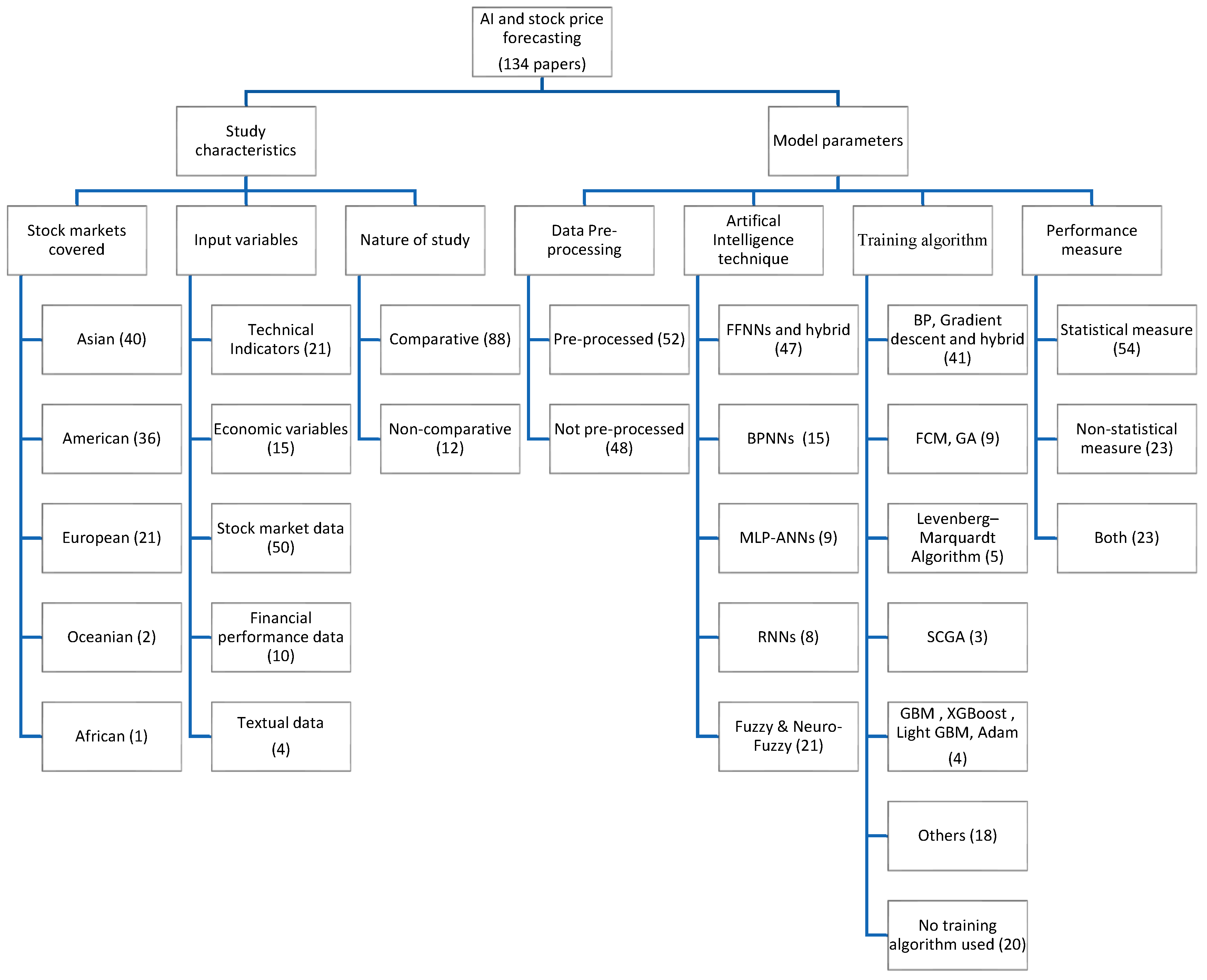
Figure 1. Organizing Framework. (Note: The percentage of papers falling into each category is mentioned in each box.).
Figure 1. Organizing Framework. (Note: The percentage of papers falling into each category is mentioned in each box.).
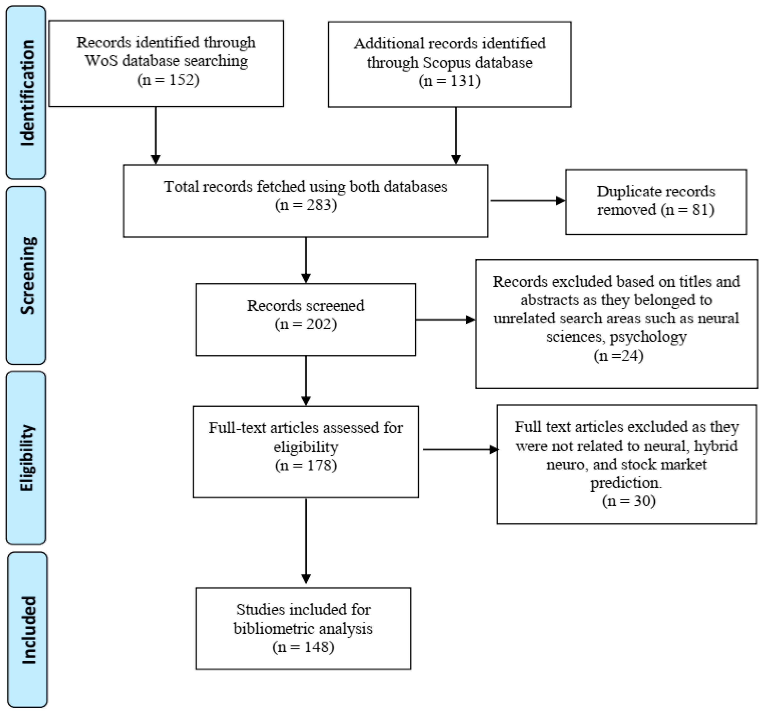
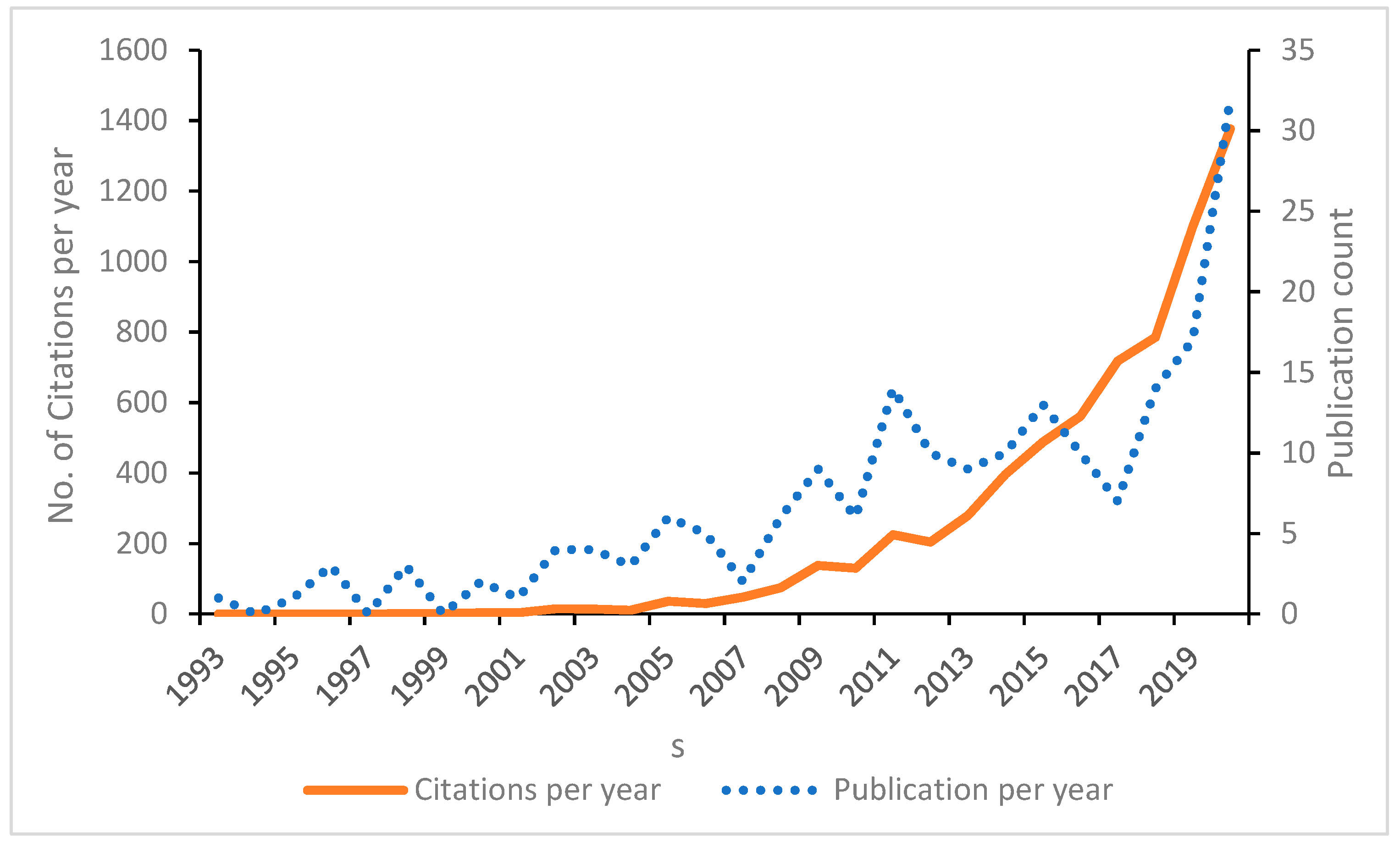
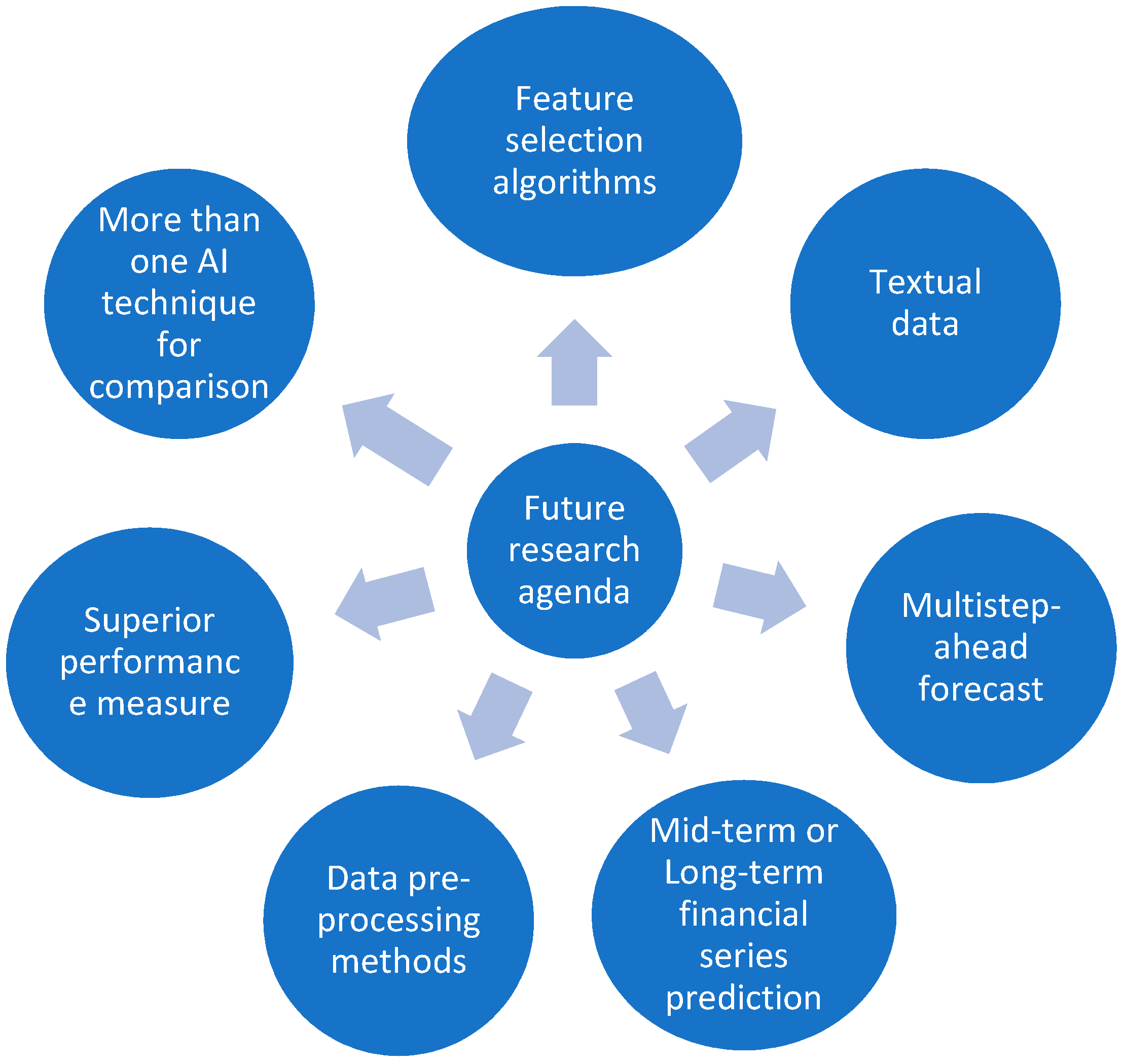
| S No. | Theme | Papers | References | S No. | Theme | Papers | References |
|---|---|---|---|---|---|---|---|
| 1 | algorithm | 111 | 609 | 23 | price | 121 | 1224 |
| 2 | analysis | 106 | 524 | 24 | problem | 91 | 362 |
| 3 | daily | 105 | 481 | 25 | process | 108 | 506 |
| 4 | data | 125 | 1489 | 26 | rate | 98 | 401 |
| 5 | error | 105 | 459 | 27 | results | 104 | 404 |
| 6 | financial | 69 | 380 | 28 | returns | 82 | 452 |
| 7 | forecasting | 106 | 890 | 29 | set | 98 | 492 |
| 8 | function | 121 | 955 | 30 | stock | 126 | 1684 |
| 9 | fuzzy | 58 | 450 | 31 | stock market | 101 | 536 |
| 10 | index | 99 | 550 | 32 | stock price | 98 | 407 |
| 11 | information | 96 | 466 | 33 | system | 101 | 692 |
| 12 | input | 120 | 711 | 34 | test | 101 | 356 |
| 13 | layer | 111 | 663 | 35 | time | 116 | 864 |
| 14 | learning | 105 | 484 | 36 | time series | 106 | 544 |
| 15 | market | 116 | 1076 | 37 | trading | 104 | 426 |
| 16 | method | 113 | 651 | 38 | training | 113 | 478 |
| 17 | model | 123 | 1633 | 39 | using | 85 | 338 |
| 18 | network | 124 | 885 | 40 | value | 119 | 854 |
| 19 | neural | 119 | 585 | 41 | variables | 100 | 656 |
| 20 | output | 119 | 615 | 42 | vector | 95 | 375 |
| 21 | parameters | 91 | 367 | 43 | weight | 93 | 350 |
| 22 | prediction | 122 | 1298 |
| Statistical Measure | Non-Statistical Measure | Both | |||
|---|---|---|---|---|---|
| Least Square Error | Guo et al. (2015); Zhongxing and Gu (1993) | Profit | Atiya et al. (1997); Ettes (2000) | Root Mean Square Error, HIT | Abraham et al. (2001); Atsalakis and Valavanis (2009b); Pantazopoulos et al. (1998) |
| Mean Square Error | Ansari et al. (2010); Casas (2001); Desai and Bharati (1998a, 1998b); Jang et al. (1991); Kim and Shin (2007) | Return | Chen et al. (2003); Gradojevic et al. (2002); Hui et al. (2000); Steiner and Wittkemper (1997) | Mc-Nemar Test, HIT | Kim and Lee (2004); Kim (1998) |
| Mean Absolute Percentage Error | Qi (1999); Abraham et al. (2004); Egeli et al. (2003) | HIT | Schumann and Lohrbach (1993); Watada (2006) | Mean Square Error, HIT | Hu et al. (2018); Koulouriotis et al. (2005); Yumlu et al. (2004) |
| Root Mean Square Error | Bildirici and Ersin (2014a); Brownstone (1996); Kanas and Yannopoulos (2001) | Sharpe Ratio | Fernández-Rodríguez et al. (2000); Armano et al. (2002) | Mean Absolute Percentage Error, HIT | Atsalakis and Valavanis (2006a, 2006b); Chun and Park (2005) |
| Mean Absolute Error | Slim (2010); Oh and Kim (2002); Yim (2002) | Direction or Trend Prediction | Harvey et al. (2000); Yiwen et al. (2000) | Root Mean Square Error, Correlation | Chen et al. (2013b); Enke and Thawornwong (2005) |
| McNemar’s Test | Kim et al. (1998); Kim and Han (2000); | Accuracy | Inthachot et al. (2016); Maknickiene et al. (2018) | Percentage of Change in Direction, Mean Absolute Percentage Error | Asadi et al. (2012); De Oliveira et al. (2013) |
| R-Square | Chaturvedi and Chandra (2004); Egeli et al. (2003); Jandaghi et al. (2010) | Sortino Ratio | Vella and Ng (2014) | Root Mean Square Error, Sharpe Ratio | Bekiros (2007); Zhou et al. (2019) |
Publisher’s Note: MDPI stays neutral with regard to jurisdictional claims in published maps and institutional affiliations.
© 2021 by the authors. Licensee MDPI, Basel, Switzerland. This article is an open access article distributed under the terms and conditions of the Creative Commons Attribution (CC BY) license (https://creativecommons.org/licenses/by/4.0/).
Chopra, R.; Sharma, G.D. Application of Artificial Intelligence in Stock Market Forecasting: A Critique, Review, and Research Agenda. J. Risk Financial Manag. 2021, 14, 526. https://doi.org/10.3390/jrfm14110526
AMA StyleChopra R, Sharma GD. Application of Artificial Intelligence in Stock Market Forecasting: A Critique, Review, and Research Agenda. Journal of Risk and Financial Management. 2021; 14(11):526. https://doi.org/10.3390/jrfm14110526
Chicago/Turabian Style